AI/ML Essentials Part 2: Cluster analysis with (Gaussian) Mixture Models#
This is the second part of the series “AI/ML Essentials”, which intends to be a gentle introduction to the topic using mostly layman’s terms and as little mathematics as possible–you don’t need an engineering degree to see the beauty within this fascinating field.
The model presented in this issue are the “Gaussian Mixture Models” (GMM) a very popular approach for cluster analysis (cf. the next section). You can find numerous introductions with code examples as well as ready-to use implementations in various programming languages. The article will again avoid formulas and too complex scientific terms and rather attempt an intuitive introduction. Whenever possible, I try to refer to the Self-Organizing Maps presented in the previous article of the series.
Enjoy reading!
Introduction#
A Taxonomy on Machine Learning#
Before me move forward to the next model, I would like to introduce some theory necessary to understand the choice of models in this series.
Machine learning can be loosely separated into four categories. This is a simplification but will serve us well for this series and each issue will correspond to one of these classes. The categories are a result of the combination of the following two properties.
- Unsupervised vs. unsupervised
In supervised learning, each observation can be separated into an input and an output quantity. After learning, a model can predict an unknown output given an input. Demand forecasting in retail and object recognition in images are good example. Unsupervised learning, however, lacks this separation, and unknown, latent (i.e., non-observable) structures or patterns are discovered in the data. Given the costs for manually labeling images for instance (think of the captchas we have to answer each day to proof we are no robots), unsupervised learning (or hybrid forms) is a very hot topic in AI/ML research.
- Symbolic vs. sub-symbolic
Categorical data consists of elements that belong to a category. Consider image recognition, for instance. The elements recognized might be “cats” and “dogs” which both belong to the category “animals”. If the output or the latent variable is categorical, we speak of symbolic learning. Sub-symbolic, on the other hand, means that the output or the latent variable are numeric in nature.
Depending on these two attributes we can distinguish the following for categories:
symbolic |
sub-symbolic |
|
|---|---|---|
supervised |
Classification |
Regression analysis |
unsupervised |
Cluster analysis |
Association & Topological analysis, dimensionality reduction |
The previous issue was dedicated to a method for topological analysis and dimensionality reduction—the Self-organizing Maps. It learns from data that is not separated (unsupervised) and it is sub-symbolic because it is strongly related the topology of the latent structure (e.g, a surface of the forearm in the example given). In today’s issue, we will remain in the domain of unsupervised learning and focus on clustering analysis. We will learn about a family of models and algorithms that are probabilistic in nature: Mixture Models.
Mixture Models: Clustering and probability distributions#
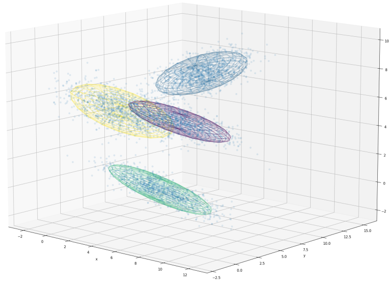
Fig. 1 Example of clustering points with Gaussian Mixture Models in 3D. Gaussian distributions can be represented by ellipsoids in 3D while in 2D, ellipses are used (see Fig. 3). In one single dimension, you would expect the iconic Bell-shaped curve.#
We should clarify the term clustering and its relation to probability distributions at first with the help of a few examples. A cluster is a group of data points that can be clearly separated from other data. It is often assumed that clusters have a unique center and and its members are distributed with a certain dispersion around it—they can be represented by a probability distribution. This is not necessarily the case for all data but if the assumption holds, mixture models work optimally. Fig. 1 shows a mixture of four clusters where the points are normally distributed. A Gaussian Mixture Model can be fit onto the data and the individual distributions that define the mixtures are visualized as ellipsoids. Humans excel in detecting clusters visually but while this ability is limited to at maximum three dimensions. Clustering analysis can operate in much higher-dimensional spaces.
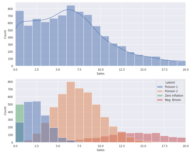
Fig. 2 Example of a mixture of different distributions in 1D. Top: A histogram of observable sales per day for a fictive SKU over a large time interval. Bottom: The (unknown) decomposition into Poisson and negative Binomial distributions as well a component of zero-inflation (e.g., missing assignments). Clustering aims at identifying the parameters of the individual components to gain hidden insights from the data.#
We are not limited, by no means, to Gaussian distributions. In Fig. 2, you can see an example that you might be more familiar with. It shows a histogram (i.e., the number of occurrences) of the number of sales per day for a single SKU. If the demand would be similar each day (independent of season and week day), we would expect a single bump following a Poisson distribution. In reality, a mixture of overlapping distributions is much more likely. The data used for the images is artificially generated, which allows showing how it is composed of multiple generating distributions. Mixture models can be fit into such data while it is much more difficult to find ready-to-use implementations than for GMM.
In the remainder of the article, we will mainly focus on GMM due to their popularity and available implementations but most concepts can be applied to different probability distributions.
Learning#
The Expectation Maximization algorithm#
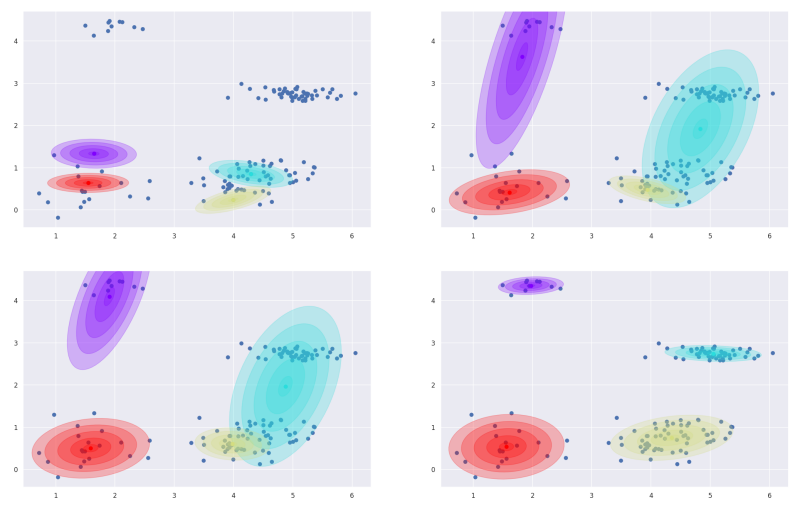
Fig. 3 Expectation Maximization algorithm for Gaussian Mixture Models. Top left: Initialization: The means and covariances of the components are are randomly chosen. Top right: First step. For each point, the probability for belonging to each cluster is computed (expectation step) and the means and covariances are updated. Bottom: After 6 and 16 steps. The algorithm converges to the correct clustering over time.#
Expectation Maximization is a very popular algorithm for learning mixture models and there is an overabundance of detailed, mathematical explanations (I found this one) to be pretty decent). Therefore, we will again skip most mathematics and just describe the two simple steps of the algorithm. The progression of learning is also depicted in Fig. 3. We start with a random initialization of the components. That is, randomly choose the mean and covariances for each Gaussian distribution. In reality, it is more efficient to have more elaborated initializations—by first applying k-means (a very simple unsupervised learning) for instance. Then we alternate between to steps until the model has converged (i.e., nothing changes anymore).
- Expectation step
Each point in the data set could theoretically be a member of each cluster. However, the further away from the center, this is less probable. A point can therefore “belong” to more than one cluster (“soft assignment”). In the expectation step, we compute the probability of cluster membership for each sample and each cluster.
- Maximization step
Based on the probabilities computed in the previous step, we can adjust our model. The parameters—means and covariances—of the individual components are recomputed such that we get more plausible distributions that better fit the data. With the updated models the cluster memberships need to be computed again too. Hence, the algorithm repeats the Expectation step.
This high-level perspective is already enough to understand and use (Gaussian) Mixture Models! The remainder of this article takes a closer look at the advantages and disadvantages of the technique and discuss the approach. If you have the time, I invite you to implement the algorithm for yourself. This is the best way of understanding how it works.
Limitations, Alternatives and extensions#
There are a number of limitations and caveats associated with learning mixture models that one needs to be aware of. Expectation maximization searches for the optimal parameter set of a mixture model given the observed data. It is therefore called a Maximum Likelihood Estimation (MLE) method. Unfortunately, a closed-form solution that allows us to easily compute solution under all circumstances does not exist and we need to resort to the alternating approach presented in the previous section. The final solution found by the algorithm therefore heavily depends on the random initialization and often enough, multiple execution is required until a satisfying solution is found. The problem intensifies with higher numbers of dimensions as suitable initializations become less likely. This limitation can be overcome by sampling-based methods that can find the unambiguous best solution by computing the Maximum A posteriori Probability distribution (MAP)1.
Another limitation is the necessity of knowing beforehand how many clusters you expect to find. While it is possible to learn with different numbers and pick the best fit, this adds additional complexity and computation time. A suitable alternative is convert the number of clusters in a random variable itself and let the learning determine its optimal value2.
Relation to other methods#
At the beginning, I described the introduced categorization as loose and in this section, I will show that the boundaries can indeed be crossed. I want to demonstrate that the world of machine learning is not that rigid and that multiple paths and customizations can lead to the best results. As they were introduced in the last issue, I will also address the Self-Organization Maps (SOM).
Self-organizing maps#
There are some similarities to the SOM, the method presented in the previous newsletter, that I want to discuss. In general, it is useful to recognize similarities and differences between the abundance of algorithms in ML and as you will see, many share similar underlying concepts and ideas. If you are not familiar with SOM, I recommend to first read the previous part in the series or skip to the next paragraph.
The most obvious commonality between SOM and GMM is that they learn from unsupervised data. While in Mixture models, however, there are prominent distributions that are not related to each other, SOM have many units that heavily influence each other. Learning too appears very different. While Expectation Maximization processes all data at once (batch learning), SOM process one sample at a time. It has not been mentioned in the first article but there is another that SOM can also be trained in batch mode. This algorithm strongly resembles expectation maximization:
Similar to the expectation step, for each sample the winning neuron of the current codebook is determined
The network is updated accounting for all samples simultaneously (summing up the updates for each sample).
Incremental learning is likewise possible with mixture models. I like to think of those methods as being cousins operating in the symbolic and sub-symbolic worlds respectively.
Supervised learning and Regression#
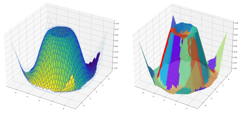
Fig. 4 Unsupervised learning for regression. Left: Self-Organizing Maps. for finding the best matching unit, only the \(x\)/\(y\) coordinates while the \(z\) value is considered as output. Right: Gaussian Mixture Models. For each \(x\)/\(y\) pair, the most likely \(z\) value can be computed.#
Mixture models and SOM are representatives of classic unsupervised learning. It might come as a surprising to learn that they can used quite conveniently for regression analysis too as shown in Fig. 4. The example shows a bi-variate, non-linear function that has been evaluated for random picks of \(x\)/\(y\) values. The resulting \(x\)/\(y\)/\(z\) triples are used as the unsupervised training data, that is, the algorithms don’t distinguish between input and output. After learning, the model can be used to generate predictions. The \(z\) component is therefore treated as a missing value, that the model fills in using its knowledge of the structure within the data.
In case of GMM, this is called Gaussian Mixture Regression. Probability theory offers the tools to compute a most likely \(z\) value given \(x\) and \(y\) through the [conditional distributions](https://en.wikipedia.org/ wiki/Multivariate_normal_distribution#Conditional_distributions) of its components. You can see in Fig. 4 that GMR resembles to covering the target surface with flat patches that are connected smoothly with each other (i.e., a local linear approximation). You can also see if you look closely that in areas with high curvature the patches are smaller. The unsupervised GMM learning excels at partitioning the data into the optimal areas. For the SOM, the best matching unit can simply be found by simply projecting the codebook vector into the \(x\)/\(y\) plane (i.e., not including \(z\) in the distance metric) and returning it’s \(z\) value. Compared to to GMR the approximation appears smooth to the eye despite predictions are discrete.
A major takeaway from this observation is that unsupervised learning can play an important (if not exclusive) role in regression tasks for feature selection or partitioning to name a few.
Dimensionality reduction#
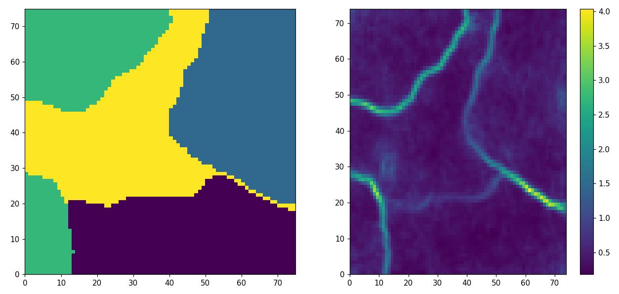
Fig. 5 Clustering with Self-Organizing Maps. The data is shown in Fig.1. (a) The grid of neuron colored according to cluster membership. The GMM of Fig.1 is used for coloring. (b) Cluster boundaries can be found measuring the distances between codebook vectors.#
Analogously, you can use SOM for clustering (see Fig 5). In that case, the som tries to fit a surface trough the clusters and large jumps between the neurons indicate cluster boundaries. The surface mainly follows the two principal axis of each cluster thus reducing the dimensionality of the feature space. While the clustering is not perfect, the dimensionality is reduced which is useful for visualization—especially when we deal with more than three dimensions—and exploration. The combination of clustering and dimensionality reduction as in Fig 5 can yield additional insights into the data.
You see, the boundaries between the categories are introduced at the beginning may be blurry and methods can be used for different purposes they have initially not been developed for.
Conclusion#
Until now, we took a close look at two specimen of unsupervised learning while focusing on their characteristics, advantages and disadvantages and much less their mathematical definition. In the upcoming issue we will venture into the world of supervised learning. We will start with regression analysis—the field which includes demand forecasting.
- 1
See the pymc3 probabilistic framework.
- 2
The model are then called Dirichlet Processes Mixture Models