AI/ML Essentials part III: Gaussian Process Regression

Introduction

In this article in the AI/ML Essentials series, we will learn about yet another machine learning model—Gaussian Process Regression. In the previous articles, we encountered instances of unsupervised learning (for clustering and density estimation). The last issue presented a simple taxonomy of machine learning, which guides us through the series:

A simple taxonomy of machine learning

	Symbolic	Subsymbolic
Unsupervised	Cluster analysis	Topological analysis, dimensionality reduction, etc.
Supervised	Classification	Regression analysis

Gaussian process regression–or GPR for short–is a representative of supervised learning. That is, a model is trained by processing data that can be divided into input and output data. Input data is equally structured as the data that is presented to the model for inference, that is, to stimulate a desired response after training. The output data, in return, is the observable response of the complex, unknown system under investigation for which we want to create a model and learn its behavior. This could be the complex customer behavior in the context of demand forecasting or complex physical systems as the weather or complex machinery, for instance. As the output is tightly coupled to the input, the terms “independent” and “dependent” variables are interchangeably used for the input and output data, respectively. We further distinguish between regression and classification in the supervised learning domain. The former produces continuous (or at least ordered) output quantities (such as the aforementioned demand forecast) from not necessarily continuous inputs, while the latter produces categorical data or symbols—much like the weather forecast warns us of “rain” or predicts “cloudy” or “sunny” skies. The boundaries, however, are not entirely fixed, and there are plenty of hybrids known—after all, your weather forecast also predicts continuous quantities such as the probability of rain at a given time. Likewise, in the domain of machine vision, algorithms can not only detect and distinguish cats from dogs (symbols) but also tell the exact pixel position in the image (continuous/ordinal).

As the name implies, we will use GPR for regression, although it can easily be extended to be used for classification tasks too. Similar to Gaussian Mixture Models (and to a less obvious extend, to the self-organizing map as pointed out in the last article), GPR is a probabilistic approach that is built upon a rich set of techniques known to the mathematical field of probability theory. Again, it revolves around the Gaussian bell curve named after the German mathematician C. F. Gauss (see Figure 1).

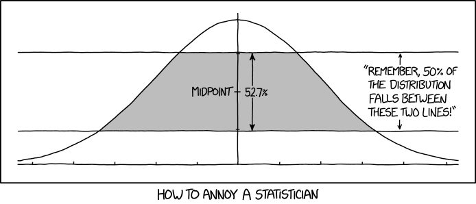
Figure 1: A not-so serious look at the Gaussian Bell function (source XKCD.com).

Gaussian Processes

GPR has two underlying concepts that are not immediately intuitive and might take a moment or two to wrap one’s head around: Gaussian processes are probability distributions over functions and are of infinite dimensionality. We will try to explore these properties in this article. In exchange, one is rewarded with another machine learning technique that can be implemented from scratch in just as little as 20-30 lines—a challenge I hope you will accept and try out on your own. Unlike the previous articles, a few formulas and python code will be included in this article.

Distributions over functions

As a quick recap, we take another look at a trained Gaussian Mixture Model as depicted in Figure 2. During training, a density function is learned that is composed of two individual Gaussian (or “normal”) distributions. Samples drawn from this mixture distributions form two clusters in the plane.

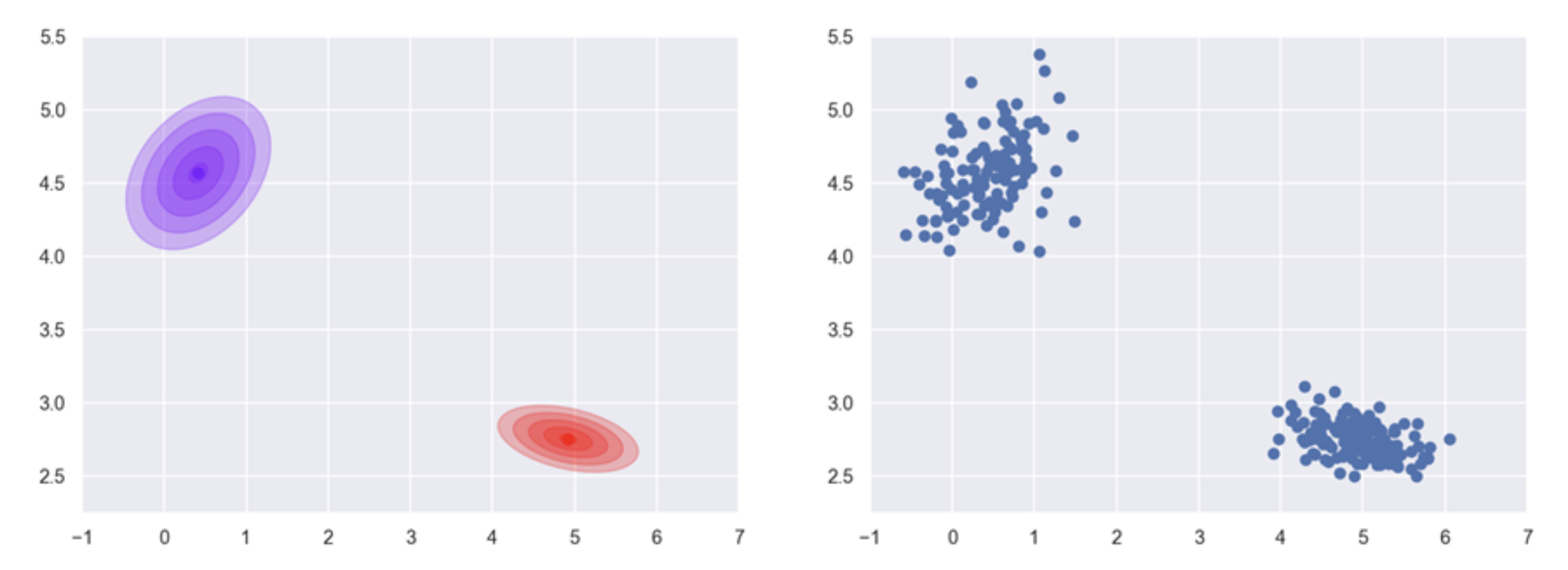
Figure 2. Drawing samples from a 2D mixture of Gaussians.

Once the parameters of the two clusters in the example have been estimated from input data (Figure 2a and 2b—remember that this is unsupervised learning), we can generate samples from randomly drawing from the two Gaussian distributions. As a crudely simplified analogy, think of the two distributions as your own two hands filled with sand. Now, let the sand trickle through your fingers, and you will end up with two small heaps on the floor that will roughly be shaped like 2D Gaussian bells. The peak of the heaps marks the most likely position where the next grain will land. Sampling from a distribution corresponds to observing the path and destination of one single, particular grain of sand.

GPR doesn’t produce single points in the Cartesian space, however. Instead, each random sample is a complete function, that is, for itself a curve or surface that maps an input to an output. Similar to the sand analogy, some functions may be more likely than others and learning in this context translates to increasing the probability of drawing functions that fit the training data optimally. As we will see in the following image, GPR grants us a good deal of control over this process.

The concept is best explained with an illustration like in Fig. 3a.

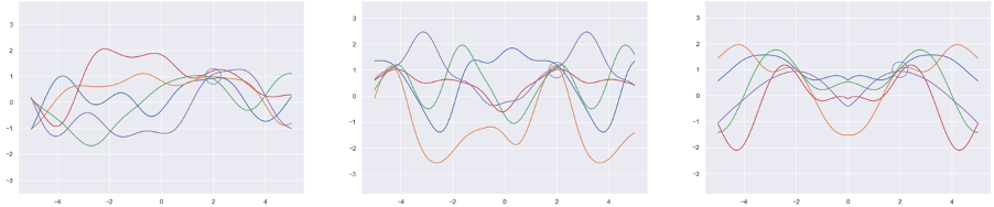
Figure 3. Examples of probability distributions over functions. One can observe that functions that pass close to the point (2,1) are more probable than others. We will see in the following how this property can be exploited for regression.

In here, you can see random functions that map an independent variable \(x\) to an independent variable \(y\). These functions belong to a random distribution; that is, some functions are more likely than others to be chosen in a random draw when sampling from the distribution. The most likely of those and \(\pm\) one standard deviation are highlighted in the graph.

When learning a target system that can be represented by a function, one first picks a distribution of a family of functions that one deems most suitable. This can be, for instance, all periodic functions with a fixed interval (Figure 3b), symmetric functions (Figure 3c), or one of the most generic cases, the family of smooth functions (Figure 3a). This choice essentially equals prior knowledge about the function that we can incorporate to improve the learning result, and we can combine this knowledge in a very flexible way. In demand forecasting, for instance, one assumes that sales on the same weekday (that is, a seven-day interval) and on the same day of the year (a 365-day interval) have a strong influence of the forecast and that the demand does not increase abruptly without a reason (smoothness). In GPR, this can be easily expressed directly in the model.

Then, training data is used to further constrain the random distribution, such that the most likely function eventually converges to the unknown target function. This process is called conditioning and is the most important step in the algorithm.

To infinity and beyond

The Gaussian distribution can be defined in a single dimension (see Figure 1)—the famous bell function—in 2D (Figure 2), in 3D (drawn as ellipsoids), or in any arbitrary, finite number of dimensions. Gaussian processes are a generalization of the Gaussian distribution to an infinite number of dimensions. This section aims at a gentle introduction to this concept, but let us start with the basics first.

Conditioning

The multivariate Gaussian distribution is defined by two things, a mean—in the example, the location of the most probable position the sand grain will land—and a covariance that decides the size and the shape of the bell. Again, in terms of the previous analogy, imagine repeating the experiment on a windy day—the bell will not be perfectly concentric but will rather resemble an ellipse.

Let’s first have a closer look at the covariance. The mean plays only a secondary role in GPR, so we will neglect it in the remainder of this article. For the 2D case, have a look at Figure 4.

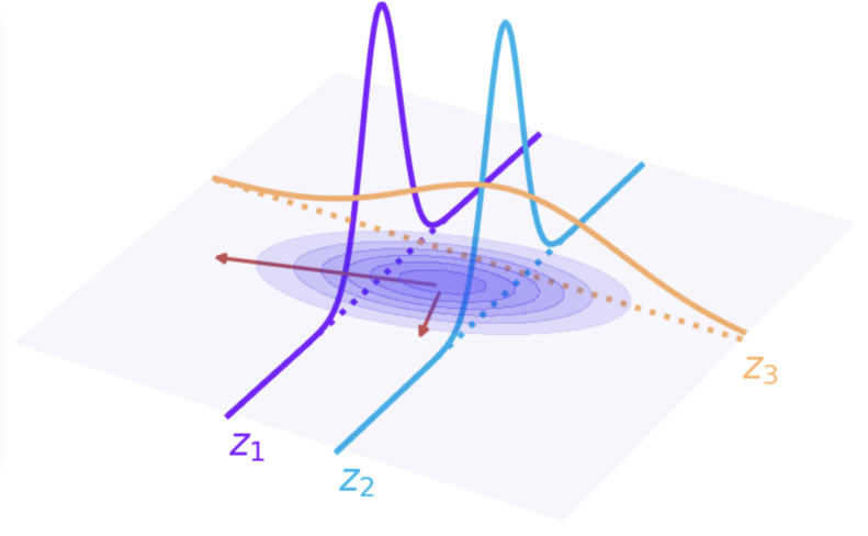
Figure 4. Conditioning of a Gaussian distribution. \(X_1\) and \(X_2\) are independent variables. There are no dependent variables as the parameter estimation of a Gaussian density (or a mixture thereof) is unsupervised learning. If \(X_1\) is set to fixed values (\(z_1\) and \(z_2\)), the remaining random variable \(X_2\) will still be distributed according to a Gaussian distribution. The same can be observed when \(X_2\) is set to \(z_3\).

Put in simpler terms, the covariance determines the rotation and the scaling among the perpendicular directions of maximal extend of the distribution—the so-called main directions. Returning to the analogy used before, if we cut the heap of sand with a knife into very, very thin, parallel slices, each slice will always have the familiar bell shape. This is always the case with Gaussian distributions.

Assigning fixed values to independent variables of a probability distribution is called conditioning and is, as mentioned earlier, a central element of GPR. When we take another look at Figure 4, we can see that the means of the distribution conditioned at the two values \(z_1\) and \(z_2\) are different. In this particular distribution, larger values along \(X_1\) occur with larger values of \(X_2\) and likewise smaller values of both values are more likely to be observed together. The two variables are correlated, and this dependency is encoded in the covariance matrix.

Correlation between training samples

Now comes the final step critical to understanding GPR. (Finite) Gaussian distributions define correlations between random variables while a Gaussian process defines a correlation between any pair of observations, that is, samples in the training data. This correlation is determined by the dependent variables, but it affects the independent variables. Think of demand forecasting and observations of one single SKU from different years. Sales from same day of week and same season are expected to experience similar sales volumes! Formally put, when two inputs \(x_1\) and \(x^\star\) are somehow similar and thus correlate, so will their associated dependent variables \(y_1\) and \(y^\star\).

While in multivariate Gaussian distributions, covariance is encoded as matrices that have to fit into a computer’s memory, a Gaussian Process defines them as a covariance function over pairs of samples such that any number of pairs can be computed without having to worry about memory constraints. This is why Gaussian Processes are considered to be infinite.

A correlation function determines how similar we think two observations are, depending on their dependent variables. There are only few restrictions on how we define this similarity between pairs of data. In Figure 4, the Euclidean distance between \(X_1\) and \(X_2\) determines the correlation. This type of correlation function results in smooth function (Figure 3a). Correlation functions are typically called “kernels,” and this particular one leading to smoothness is called squared exponential kernel. Periodic functions are enforced when the kernel includes trigonometric functions. Symmetry is achieved by comparing distances with the common symmetry axis.

Learning with GPR

In the previous section, we have learned that we can define correlations between observations within a dataset. In the training set, we know the dependent variables while during inference (when we try to predict), these are unknown.

For learning, we first define a Gaussian process over this data by choosing a suitable covariance function. For each element of the inference dataset, we then constrain the process on all dependent variables in the training dataset and the element (a dependent variable) itself. The Gaussian process might be infinite, but after constraining, we always get a regular multivariate Gaussian with a finite covariance matrix. In practice, we have to deal only with standard Gaussian functions in our computations. Now, we know the correlation between the element and each observation of the training dataset. From that, we can easily compute the most likely response to the element with the tools applicable to multivariate Gaussian distributions. The resulting value is what we use as our prediction. We repeat the same steps for the remaining elements in the inference dataset.

Once these steps are clear, the implementation is very straightforward. All formulas for conditioning and handling multivariate Gaussian densities are well known and easy to implement. The formulation of the kernels used in the covariance function is simple and can be chosen from a range of readily available candidates. In the next section, we will go through a very basic implementation in the Python programming language—feel free to skip this rather technical part if you like.

Implementation

In this section, we have a look at a minimal implementation of GPR in the Python programming language. Therefore, the next paragraphs will be very technical and include programming code. For the understanding of the method, this is not mandatory, but it helps to see how quickly a working prototype can be generated. If you are interested in programming, I recommend you try to implement it for yourself first.

Conditioning

We start with small helper artifact—a decorator—which a little boilerplate abstraction that takes care of bringing the parameters in the correct shape and compute correlation matrices such that we can focus on the actual kernels and the overall implementation becomes more compact. The mathematical interpretation meaning is shown on the right. Note that we restrict ourselves to univariate regression in this section. For the multivariate case, the code needs to be adapted.

A decorator to define kernel functions

import numpy as np

def kernel_function(f):
    def decorator(x, y, *args, **kwargs):
        xx, yy = np.meshgrid(x, y)
        val = f(xx, yy, *args, **kwargs)
        return val

    return decorator

(1)\[\begin{split}k\left((x_1,x_2)^T,(y_1,y_2)^T\right) \rightarrow \begin{pmatrix} k(x_1,y_1) & k(x_1,y_2) \\ k(x_2,y_1) & k(x_2,y_2) \end{pmatrix}\end{split}\]

Then, we define a function that computes the conditional distributions for us. This function expects a kernel function, an array of sites x for prediction (here a fine granular range for plotting), and training data (\(X\), \(Y\)). It returns the means and variance and a confidence interval plotting (i.e., used for the color bands in the following plots).

Evaluating a GPR by conditioning.

def gpr(kernel, x, X, Y, noise=0):
    cov_X = kernel(X, X) + np.identity(len(X)) * noise
    cov_Xx = kernel(x, X)
    cov_x = kernel(x, x)

    mean = (cov_Xx.T @ np.linalg.inv(cov_X) @ Y.reshape(-1, 1)).flatten()
    var = cov_x - cov_Xx.T @ np.linalg.inv(cov_X) @ cov_Xx

    upper = mean + var.diagonal()
    lower = mean - var.diagonal()

    return mean, var, upper, lower

(2)\[\begin{split}\begin{aligned} \mu_x &= k(x, X)^T \cdot k(X,X)^{-1} \cdot Y^T \\ ~ \\ \Sigma_x &= k(x , x ) - k(x , X)^T \cdot k(X,X)^{-1} \cdot k(x , X) \end{aligned}\end{split}\]

Kernel functions

We can now focus on the actual kernels! We will look at the three examples we already have seen in Figure 3—the squared exponential kernel for smooth functions, a periodic and a symmetric kernel. Implementing a kernel is actually very simple. One only needs to express the respective formulas over two parameters (vectors) \(x\), \(y\).

@kernel_function
def squared_exponential(x, y):
    return np.exp(-((x - y) ** 2) / 2)

(3)\[k(x,y) = \exp\left( -\frac{(x-y)^2}{2} \right)\]

@kernel_function
def periodic(x, y):
    return np.exp(np.cos((x - y)))

(4)\[k(x,y) = \exp(\cos(d))\]

@kernel_function
def symmetric(x, y):
    return np.exp(-((abs(x) - abs(y)) ** 2) / 2)

(5)\[k(x,y) = \exp\left(-\frac{(|x|-|y|)^2}{2}\right)\]

We can now investigate the behavior of the different kernels as shown in Figure 5. There, we try to train a GPR to predict sinus signal. In the upper image, the squared exponential kernel achieves a very good interpolation between the given examples (indicated as dots on the sinus function). The variance is very on the predicted curve between these points as indicated by the confidence interval (i.e., the transparent color band). The middle image displays what happens if we use a periodic kernel. We expect that this kernel is better suited and in fact, in addition to a good interpolation, the prediction for sites that are far from the training samples (e.g., \(x=4.5\)) are very good. Finally, the symmetric kernel gives wrong predictions with a high confidence! This is little surprising—the target function is not symmetric after all. I recommend you go ahead and explore the behavior on more interesting examples!

Use can use this code snippet to generate the plots:

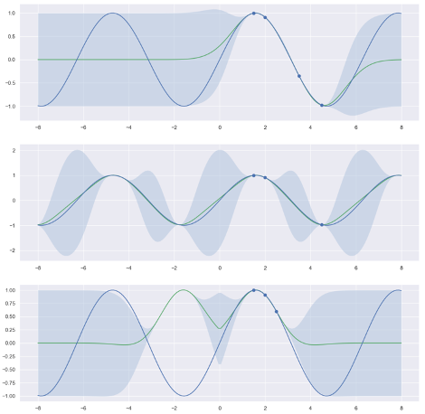
Figure 5: Regression with three different kernels for a sinus target. Top: squared exponential kernel. Middle: Periodic kernel. Bottom: Symmetric kernel.

Limitations

One important aspect of GPR that distinguishes it from other learning methods (neural networks, for instance) is the fact that it does not require a dedicated learning phase. All computation is conducted during inference—the moment when we try to get a prediction. This is called lazy learning. While we obviously save the time of learning, inference is much more expensive, which, in practice, is a limiting factor for the application of GPR. Inference involves the expensive operation of matrix inversion (cubic complexity) applied to a matrix that grows in the size of training data, and some efforts might be required to maintain acceptable computation times. These properties affect the range of application—even if there are remedies for these problems. GPR, however, is a fascinating tool for exploring smaller datasets and plays an important role in Bayesian analysis as a prior for functions. Finally, GPR—as the name implies—assumes a normal distributed (that is, Gaussian) noise. In many domains that involve countable observations (such as sales in demand predictions) where non-negative values cannot occur, GPR cannot be directly deployed unless only very large numbers are involved and natural zeros cannot occur.

Conclusion

GPR is a powerful regression technique, and it allows data scientists to include a lot of prior domain knowledge at little costs. It therefore grants a high degree of explainable influence on the model. However, the theory behind them is often considered repelling or even intimidating at the beginning due to its deep roots in probability theory. The reader, however, might find it refreshing to see that this complex definition still translates to a very clean, compact, and concise implementation.

In the next release of the AI/ML series, we will explore another supervised learning algorithm, this time to solve classification tasks.

AI/ML Essentials Part 2: Cluster analysis with (Gaussian) Mixture Models